Excel is extremely useful program to create spreadsheets, with many functions for various calculations and reporting ... But, sometimes after long and hard work it turns out the ideal table of sheets is 10, but you need to fit everything on one sheet.

Luckily, the program has the ability to customize your spreadsheet to get everything on one page and make it look as perfect as possible. If your spreadsheet is too big for one page, you can use these settings to neatly spread it across multiple pages.

PREVIEW BEFORE PRINTING

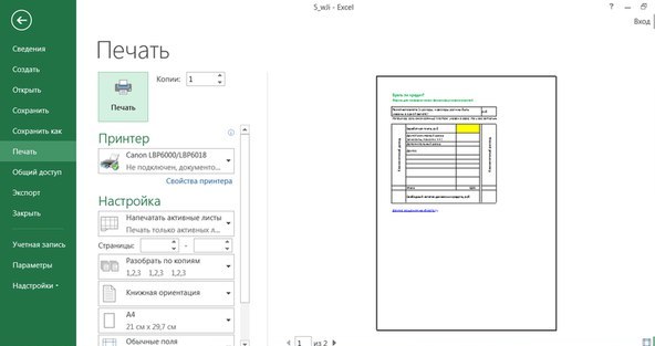
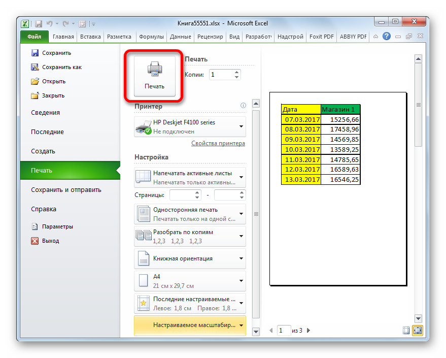
This important function, without which you would have to print everything, just to check how the table looks on the sheet, while spending a lot of time and paper. With the help of the preview you can see how the printed document will look, and at this stage you can still make various changes to make everything look neater...

Unfortunately, Excel has changed its structure and in its various versions you need to enter the preview in different ways: file => print => preview; or file => print and see what your table will look like. If everything suits you, then go ahead and print the document. If not, try one of the strategies listed below.

CHANGING PAGE ORIENTATION

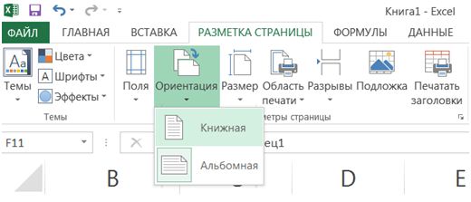
If your table is very wide, it is better to choose horizontal page orientation. If it is very high - vertical. To choose orientation: open page options => select portrait or landscape; also orientation can be in "page layout" => orientation.

DELETE OR HIDE ROWS (COLUMNS)

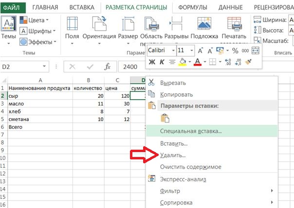
Large tables often have rows or columns that contain old information, or information that is not required to be printed. These unnecessary rows and columns take up valuable space on the page, and may be the reason why all the information doesn't fit on one sheet. If you have rows or columns that you can delete - select them => right click => select "delete".

If you think they contain information that will be needed again someday, you can hide them by right-clicking on a column or row header and selecting "hide". To display the data again - select the columns or rows on both sides of the hidden ones, and right-click => "show".

USE A PAGE BREAK

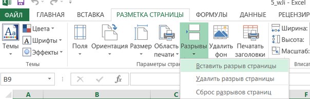
As well as in text editor, in Excel you can make a page break, while you choose where it is better to do it. To do this, select the right place and use the "page markup", then select the breaks. Page breaks are inserted above and to the left of the selection.

CHANGING THE PRINT AREA

If in your table great amount information, and you need to print only part of it, then select the desired fragment, click "Print", and then select "print the selected fragment" in the settings.

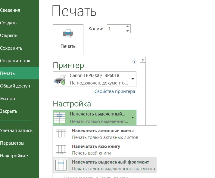
You can also specify the page numbers you want to print, or select other print options.

CHANGING PAGE MARGINS

If you do not have enough space to fit the table on a piece of paper - then you can add extra bed using fields. To do this, go to the "Page Options" menu and select the "Margins" column.

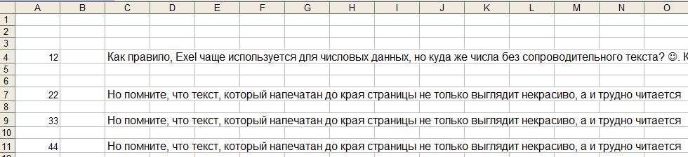
But remember that text that is printed to the edge of the page not only looks ugly, but is also difficult to read.

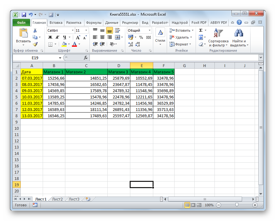
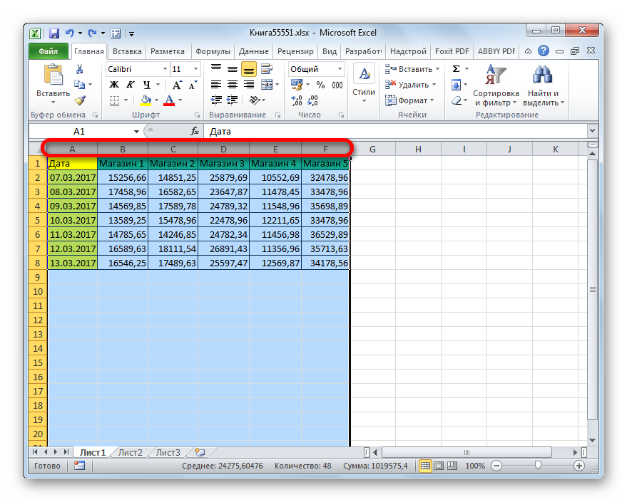
RESIZE COLUMNS

As a rule, Excel is more often used for numeric data, but where are numbers without accompanying text? Which is sometimes a lot, which in turn often makes it difficult to place a table on one page, or at least on several.

some text juts out far to the right and enlarges the document by several pages accordingly. Another way to reduce the size of your document is to reduce the width of your columns, but be sure you don't lose the data you want to print. To do this, go to the alignment menu and turn on text wrapping. (in some Excel, you need to right-click on a cell => cell format => alignment tab => word wrap)

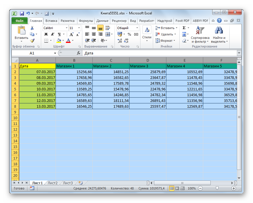
now when the text does not go beyond the column - you can expand the size of the column simply by dragging the edge of the header.

SCALING TABLES

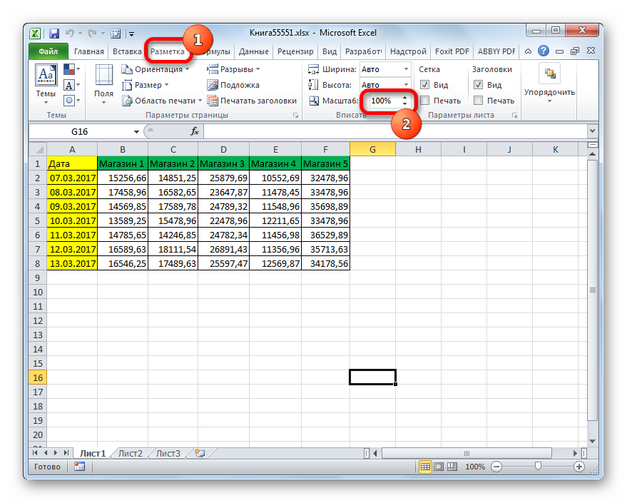
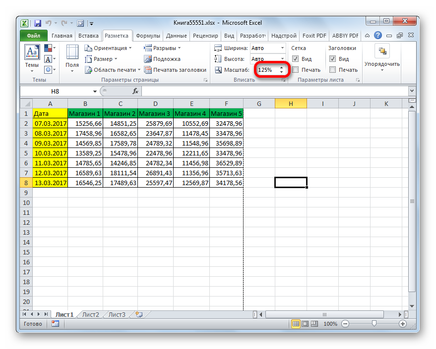
You can scale the table to fit the page, or a certain amount pages. In Page Options, select the number of pages you want to print. Choice fewer Pages Width will scale pages horizontally by choosing fewer pages tall - vertically. You can also zoom in or out by percentage.

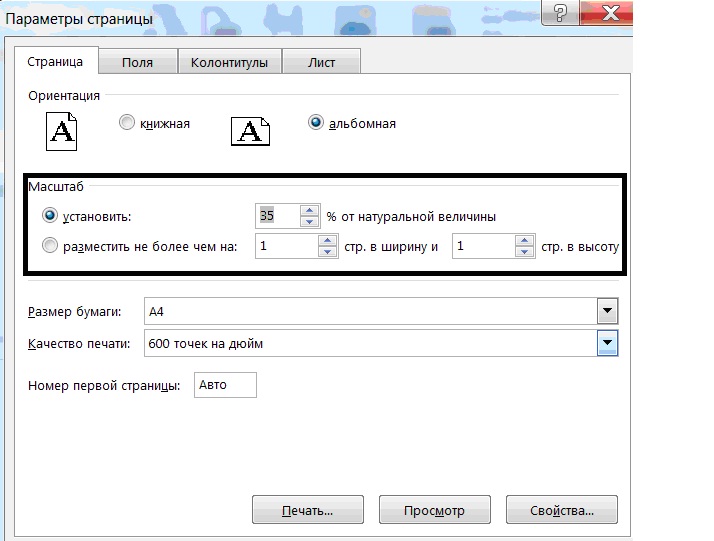
Using the scaling option can help you fit the right sign on the sheet of paper, but don't forget to preview it before you print, because you can reduce everything to hard to read.

There are many more useful functions in Excel, but we will talk about them next time. If there are additions - write comments! Good luck to you 🙂

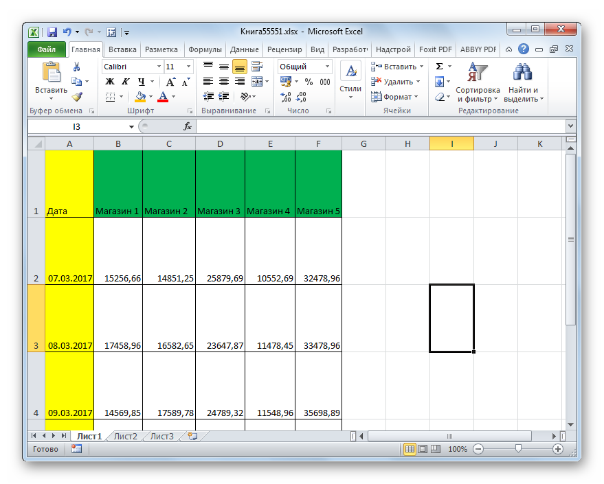
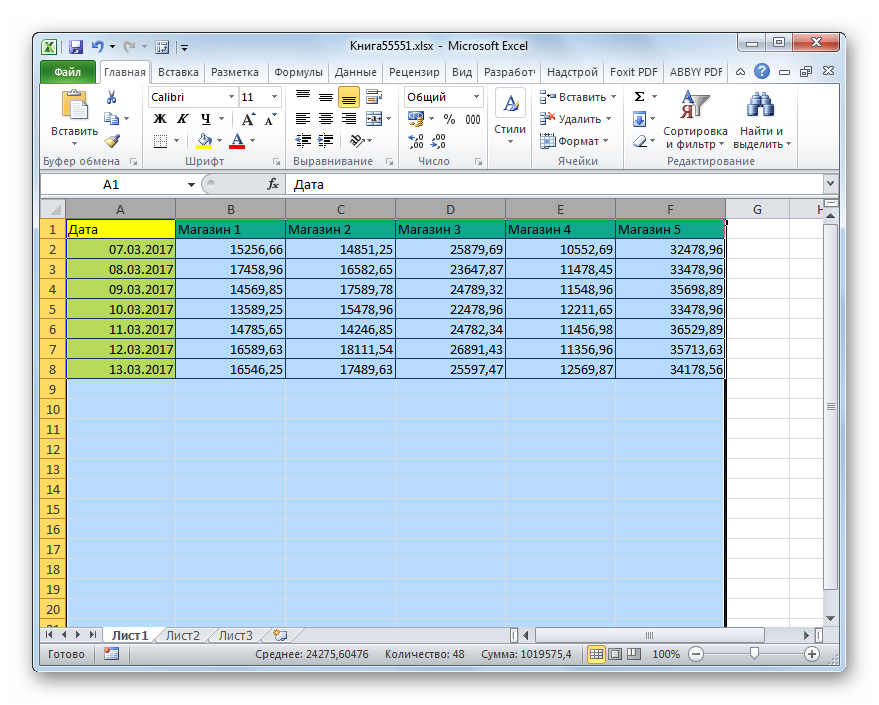
When working with spreadsheets sometimes you need to increase their sizes, because the data in the resulting result is too small, making it difficult to read. Naturally, each more or less serious word processor has in its arsenal tools to increase the table range. So it is not at all surprising that such a multifunctional program as Excel also has them. Let's see how in this application you can increase the table.

It must be said right away that there are two main ways to enlarge a table: by increasing the size of its individual elements (rows, columns) and by applying scaling. In the latter case, the table range will be increased proportionally. This option splits into two separate ways: Zoom on screen and print. Now let's look at each of these methods in more detail.

Method 1: increase individual elements

First of all, let's look at how to increase individual elements in a table, that is, rows and columns.

Let's start by increasing the rows.

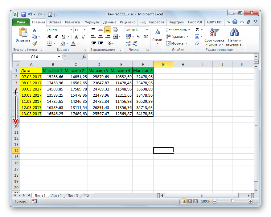
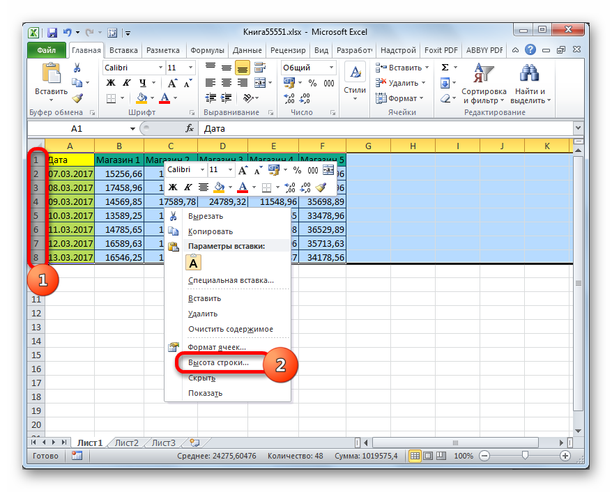
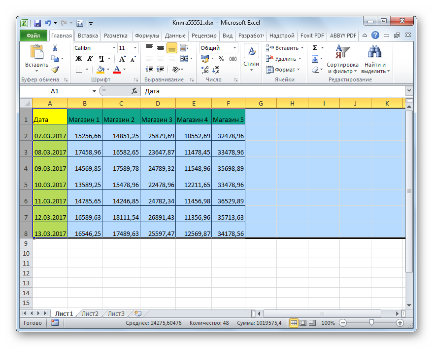
Sometimes it is required to expand not one row, but several rows or even all rows of a tabular data array, for this we perform the following steps.

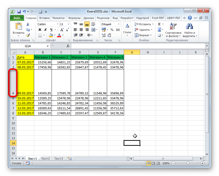
There is also another option for string expansion.

Now let's move on to options for increasing the table array by expanding columns. As you might guess, these options are similar to those with which we increased the height of the lines a little earlier.

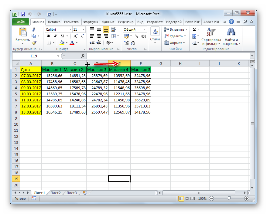
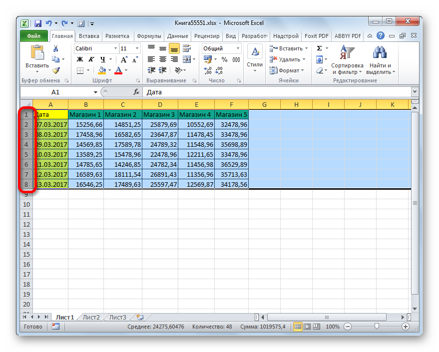
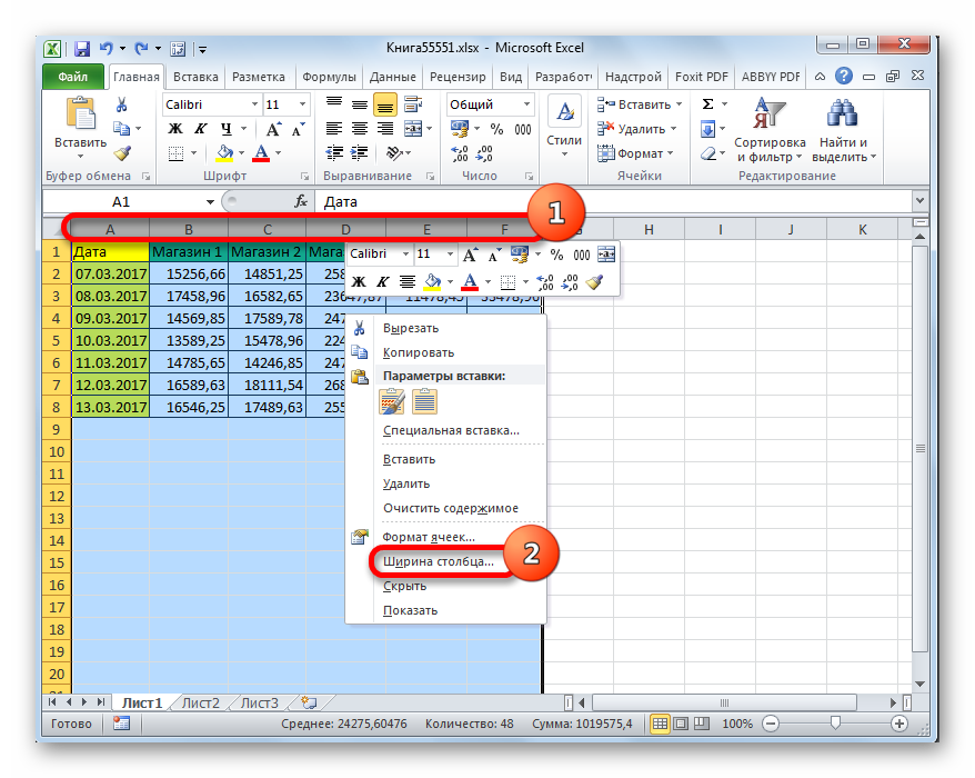
As in the case of rows, there is an option to bulk increase the width of columns.

In addition, there is an option to increase the columns by entering their specific value.

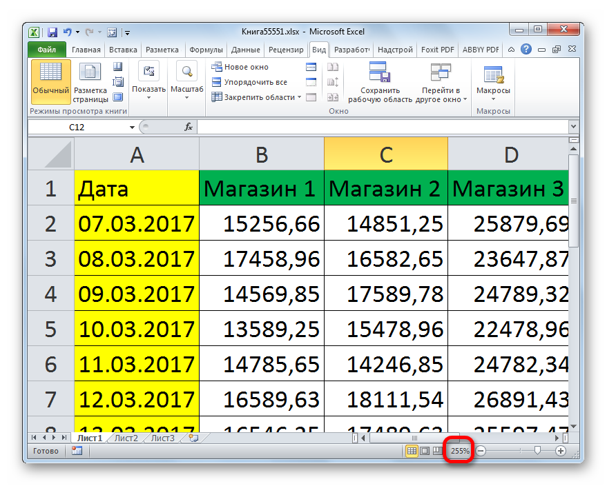
Method 2: scaling on the monitor

Now let's learn about how to increase the size of a table by scaling.

It should be noted right away that you can scale the table range only on the screen, or on a printed sheet. Let's look at the first of these options first.

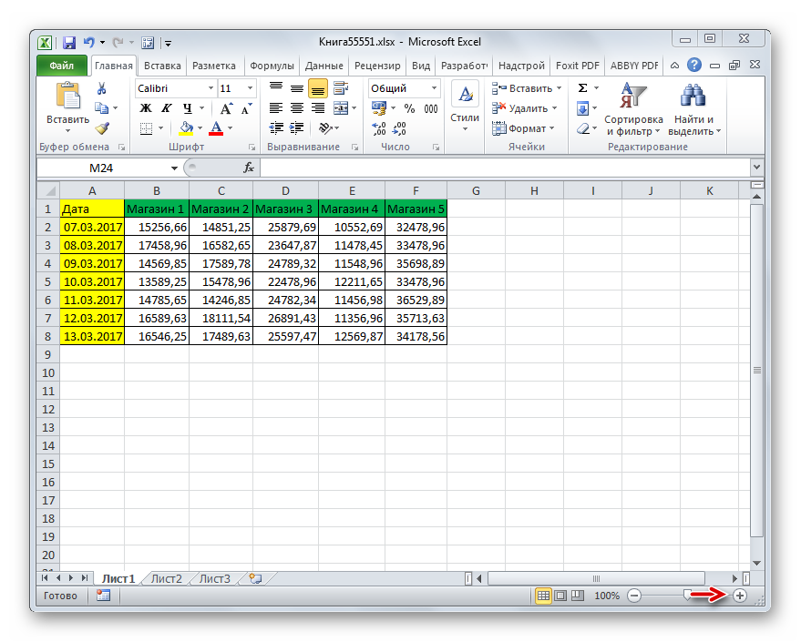
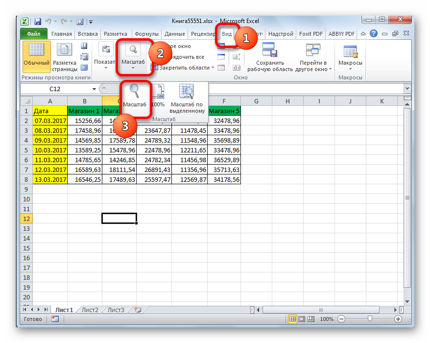
In addition, the scale displayed on the monitor can be changed as follows.

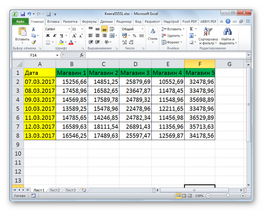
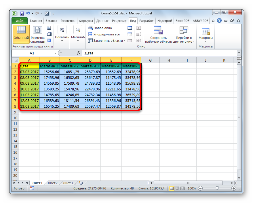
Quite a useful tool "Zoom by selection", which allows you to zoom in on the table just enough so that it fits completely into the area of ​​​​the Excel window.

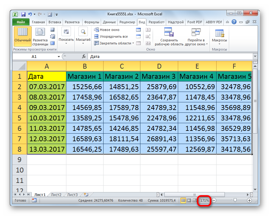
In addition, the scale of the table range and the entire sheet can be increased by holding the button ctrl and scrolling the mouse wheel forward (“away from you”).

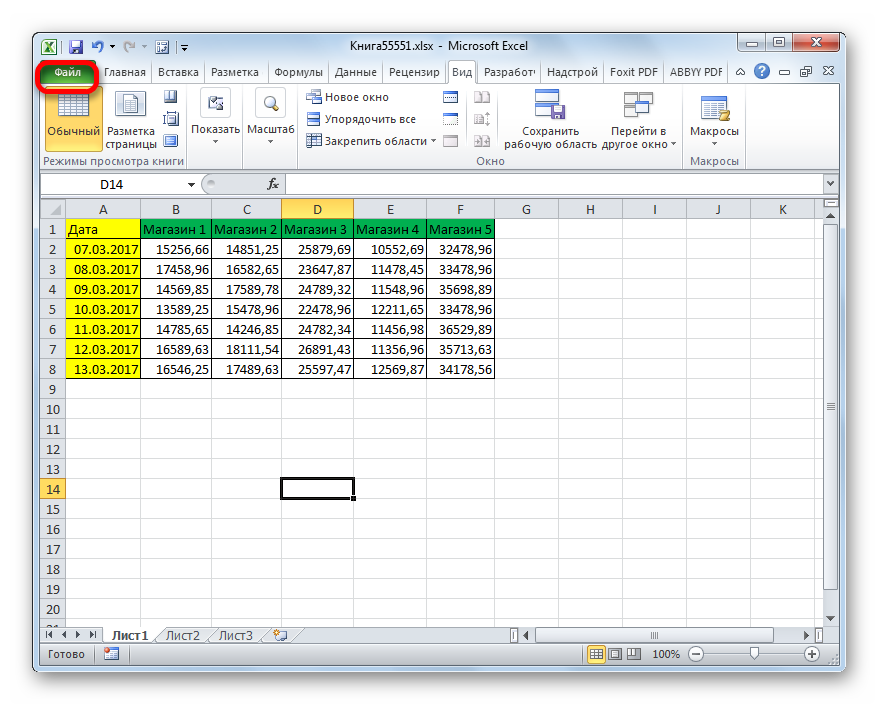
Method 3: rescaling the table on print

Now let's see how to change real size table range, that is, its print size.

You can change the scale of the table when printing in another way.

As you can see, you can enlarge a table in Excel different ways. And the very concept of increasing the table range can mean completely different things: expanding the size of its elements, zooming in on the screen, zooming in on print. Depending on what the user this moment need, he must choose specific option actions.

When working in Excel, some tables reach a rather impressive size. This leads to the fact that the size of the document increases, sometimes reaching even a dozen megabytes or more. Increasing the weight of an Excel workbook leads not only to an increase in the amount of space it takes up on the hard drive, but, more importantly, to a slowdown in execution speed various activities and processes in it. Simply put, when working with such a document, Excel starts to slow down. Therefore, the issue of optimizing and reducing the size of such books becomes relevant. Let's see how you can reduce the file size in Excel.

An overgrown file should be optimized in several directions at once. Many users do not realize, but often an Excel workbook contains a lot of unnecessary information. When the file is small, no one pays much attention to this, but if the document has become unwieldy, you need to optimize it in all possible ways.

Method 1: reduce the operating range

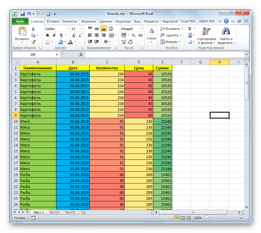
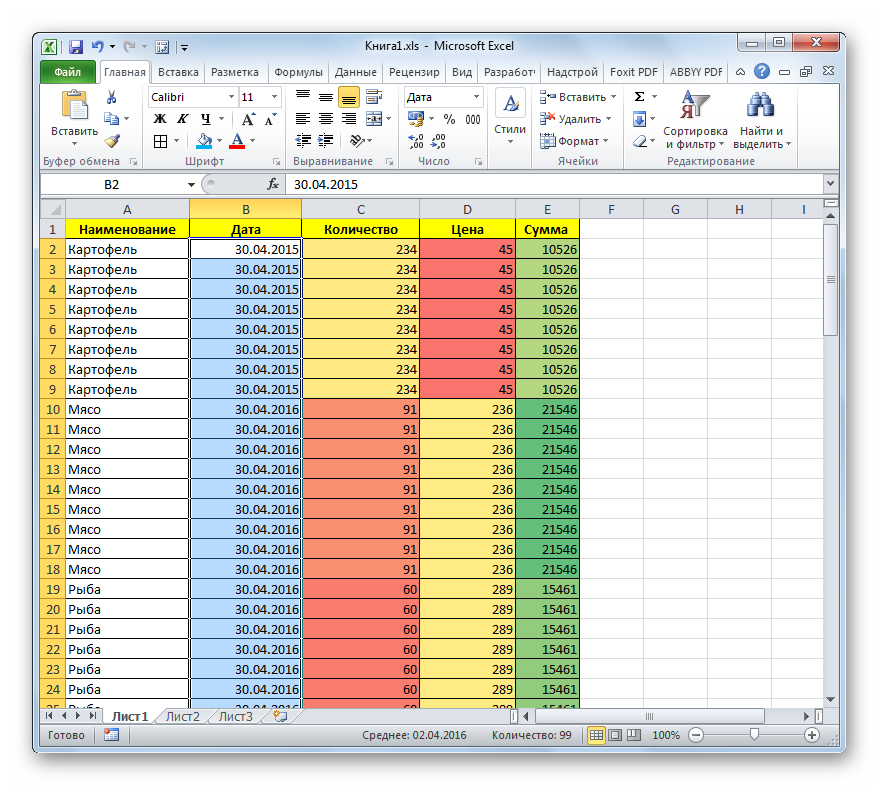
The working range is the area in which Excel remembers the actions. When recalculating a document, the program recalculates all cells in the workspace. But it does not always correspond to the range in which the user actually works. For example, an inadvertently placed space far below the table will expand the size of the working range to the element where this space is located. It turns out that Excel will process a bunch of empty cells each time when recalculating. Let's see how we can fix it this problem on the example of a specific table.

If there are several sheets in the book that you work with, you need to carry out a similar procedure with each of them. This will further reduce the size of the document.

Method 2: Eliminate redundant formatting

Another important factor that makes Excel document more severe is redundant formatting. This may include the use various kinds fonts, borders, number formats, but first of all it concerns cell filling different colors. So before you further format the file, you need to think twice about whether it is necessary to do this or you can easily do without this procedure.

This is especially true for books containing a large number of information, which in itself already have a considerable size. Adding formatting to a book can even increase its weight by several times. Therefore, you need to choose the "golden" mean between the visibility of the presentation of information in the document and the file size, apply formatting only where it is really necessary.

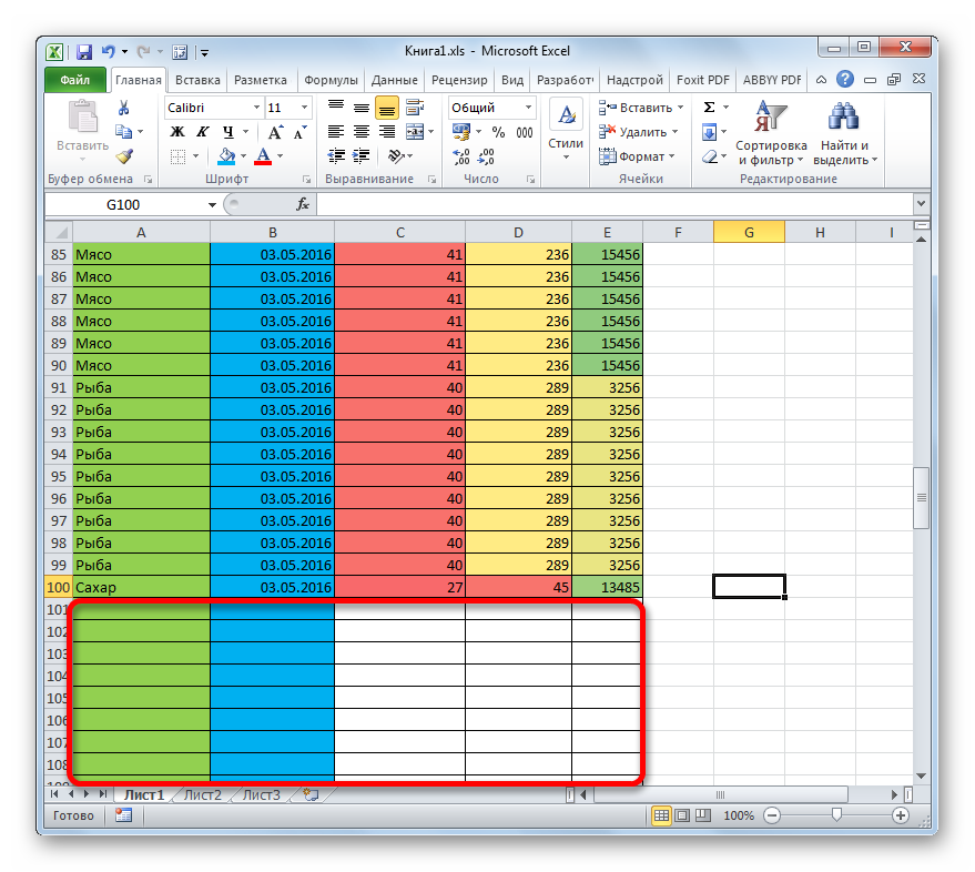
Another factor that adds weight to formatting is that some users prefer to format cells "oversized". That is, they format not only the table itself, but also the range below it, sometimes even to the end of the sheet, with the expectation that when new rows are added to the table, it will not be necessary to format them again each time.

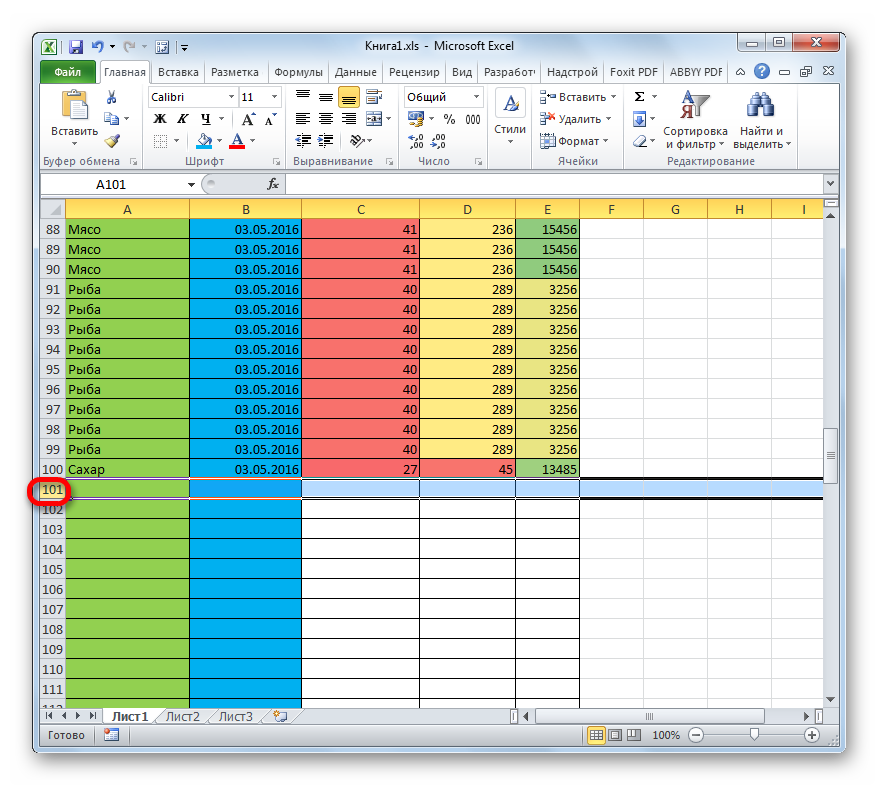
But it is not known exactly when new lines will be added and how many of them will be added, and by such preliminary formatting you will make the file heavier right now, which will also negatively affect the speed of working with this document. Therefore, if you applied formatting to empty cells not included in the table, then it must be removed.

The above steps will help to significantly reduce the size of an Excel workbook and speed up work in it. But it is better to initially use formatting only where it is really appropriate and necessary, than to spend time on optimizing the document later.

Method 3: Remove Links

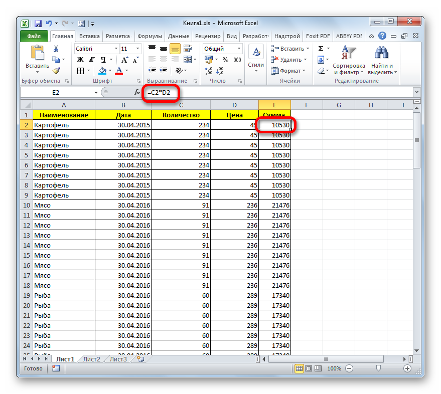
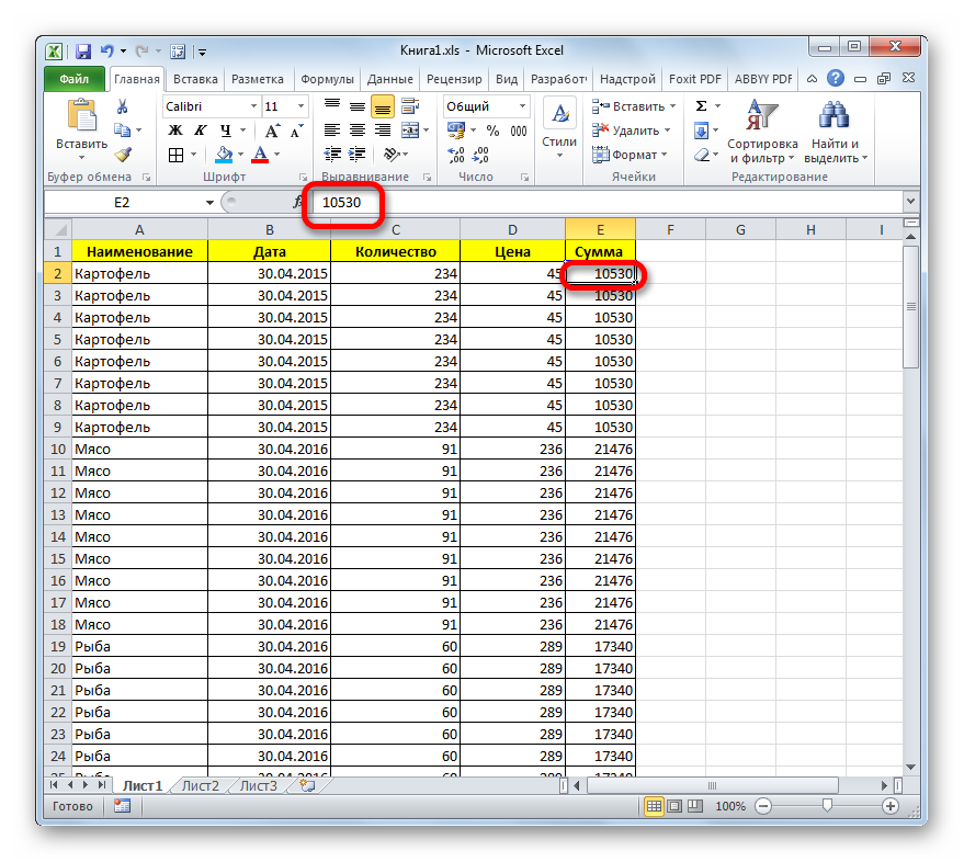
In some documents, there are a very large number of links from which values ​​are pulled up. This can also seriously slow down the speed of work in them. This show is especially affected by external links to other books, although internal links also have a negative impact on performance. If the source from which the link takes information is not constantly updated, that is, it makes sense to replace the link addresses in the cells with normal values. This can increase the speed of working with the document. You can see if the link or value is in a particular cell in the formula bar after selecting the element.

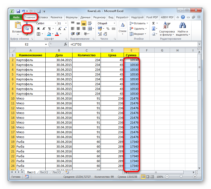
But you need to remember that this option for optimizing an Excel workbook is not always acceptable. It can only be used when the data from the original source is not dynamic, that is, it will not change over time.

Method 4: format changes

Another way to significantly reduce the file size is to change its format. This method, probably, helps to compress the book more than anyone else, although the above options should also be used in combination.

There are several "native" file formats in Excel - xls, xlsx, xlsm, xlsb. The xls format was the base extension for Excel 2003 and earlier. It is already obsolete, but, nevertheless, many users continue to use it to this day. In addition, there are times when you have to go back to working with old files that were created many years ago, back in the days of the absence of modern formats. Not to mention the fact that many third-party programs work with books with this extension, which are not able to process later versions of Excel documents.

It should be noted that a book with xls extension has much larger size than its modern analogue of the xlsx format, which Excel currently uses as the main one. First of all, this is due to the fact that xlsx files, in fact, are compressed archives. Therefore, if you use the xls extension, but want to reduce the weight of the book, then this can be done simply by resaving it in the xlsx format.

In addition, in Excel there is another modern xlsb format or a binary book. It saves the document in binary encoding. These files weigh even less than xlsx books. In addition, the language in which they are written is closest to Excel programs. Therefore, it works with such books faster than with any other extension. At the same time, the book of the specified format is in no way inferior to the xlsx format in terms of functionality and possibilities of using various tools (formatting, functions, graphics, etc.) and surpasses the xls format.

The main reason why xlsb has not become the default format in Excel is that third-party programs practically cannot work with it. For example, if you need to export information from Excel to the 1C program, then this can be done with xlsx or xls documents, but not with xlsb. But, if you do not plan to transfer data to any third-party program, then you can safely save the document in xlsb format. This will allow you to reduce the size of the document and increase the speed of work in it.

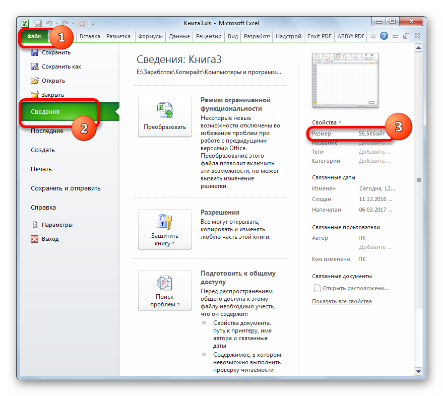
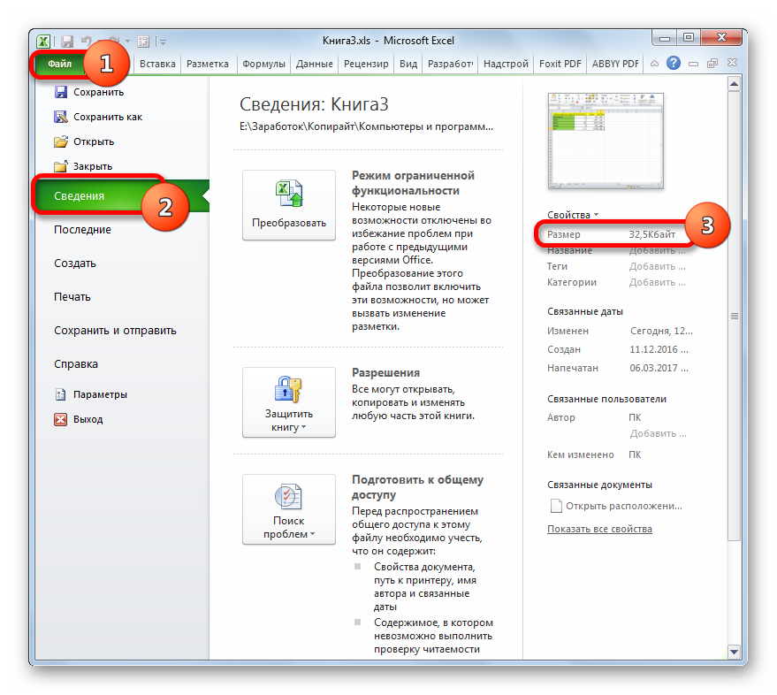
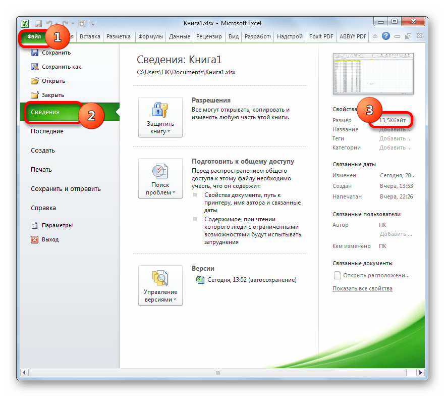
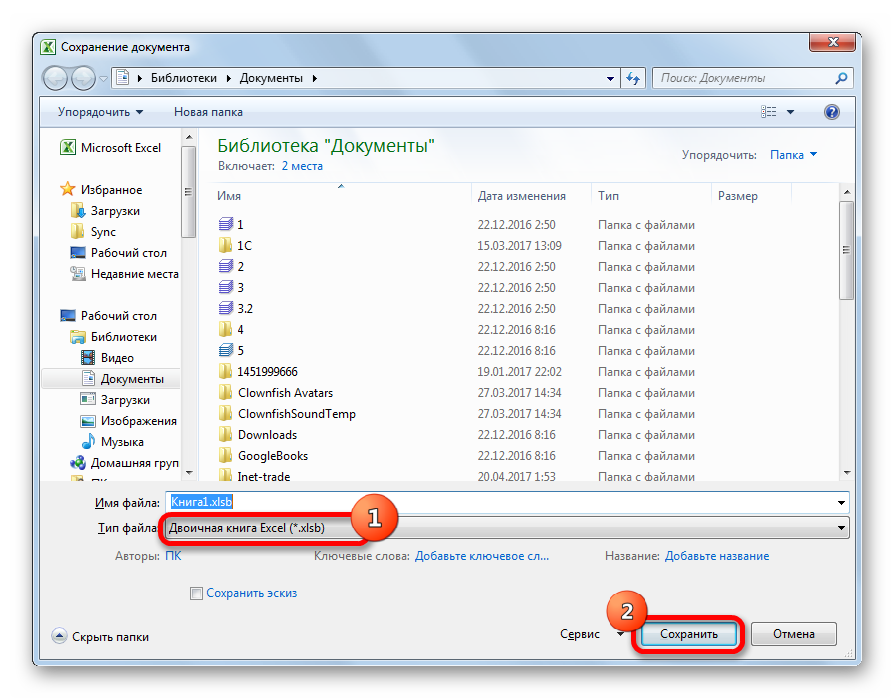
The procedure for saving a file in the xlsb extension is similar to what we did for the xlsx extension. In the tab "File" click on item "Save as…". In the save window that opens, in the field "File type" you have to choose an option "Excel Binary Workbook (*.xlsb)". Then click on the button "Save".

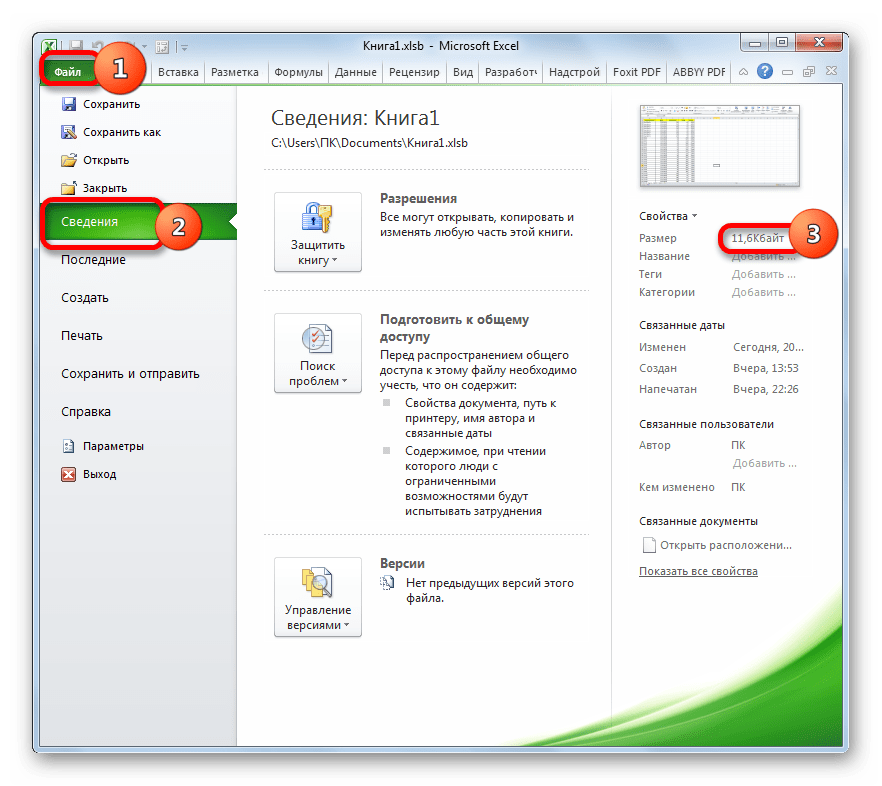
We look at the weight of the document in the section "Intelligence". As you can see, it has decreased even more and now it is only 11.6 KB.

Summing up, we can say that if you work with a file in xls format, then the most effective way to reduce its size is resaving in modern xlsx or xlsb formats. If you are already using these file extensions, then to reduce their weight, you should properly configure the workspace, remove redundant formatting and unnecessary links. You will get the greatest return if you perform all these actions in a complex, and not limit yourself to only one option.

When you create documents for printing (for example, reports, invoices, invoices, etc.), it is important to set them up so that the printed sheet looks correct, convenient and logical. What worksheet settings you can do - I will tell in this post.

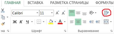
Most of the settings can be made in the " Page settings". It is called by clicking on the icon in the corner of the ribbon block Page Layout - Page Setup .

Page Setup icon

Page Orientation in Excel

Depending on the shape of the data on the sheet, you can choose portrait (vertical) or landscape (horizontal) orientation. You can do this in the following ways:

1. Complete tape command Page Layout - Page Setup - Orientation . In the menu that opens, select one of the two options
2. Complete File - Print , in the print settings window you can also choose the orientation

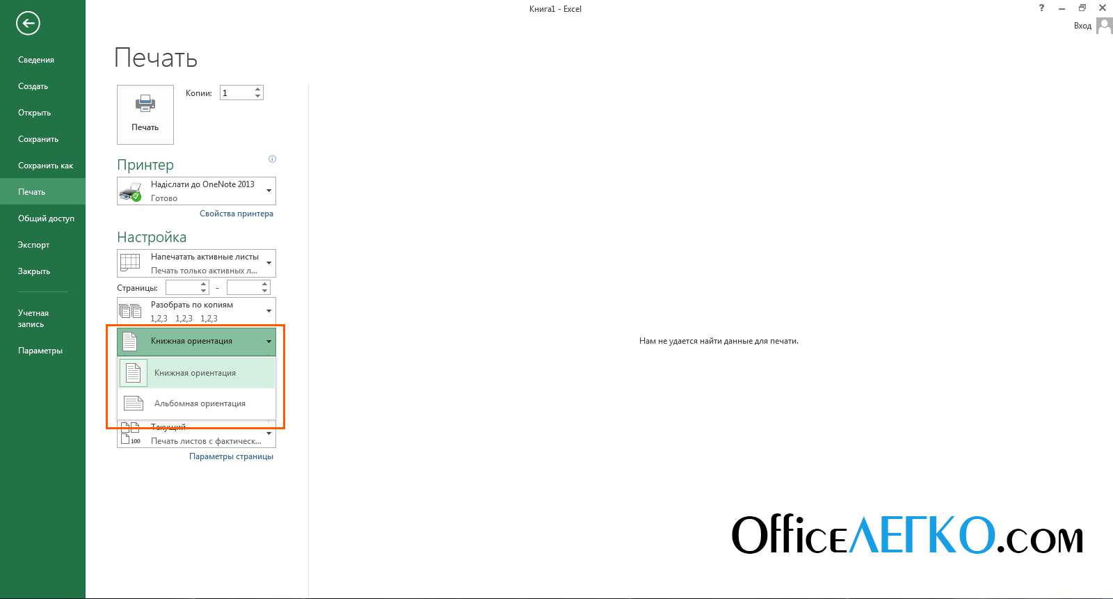
Setting the paper orientation

1. In the dialog box " Page settings» tab « Page', block ' Orientation» — select the radio button you want

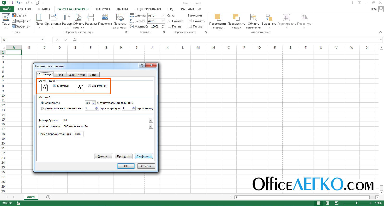
Orientation in Page Setup

Each of these methods will change the orientation of the active sheet, or all selected sheets.

How to change page size in excel

Although most printers print on A4 (21.59 cm x 27.94 cm) sheets, you may need to change the size of the printed sheet. For example, you are preparing a presentation on A1 sheet, or you are printing branded envelopes of appropriate sizes. To resize a sheet, you can:

1. Use the command Page Layout - Page Setup - Size .

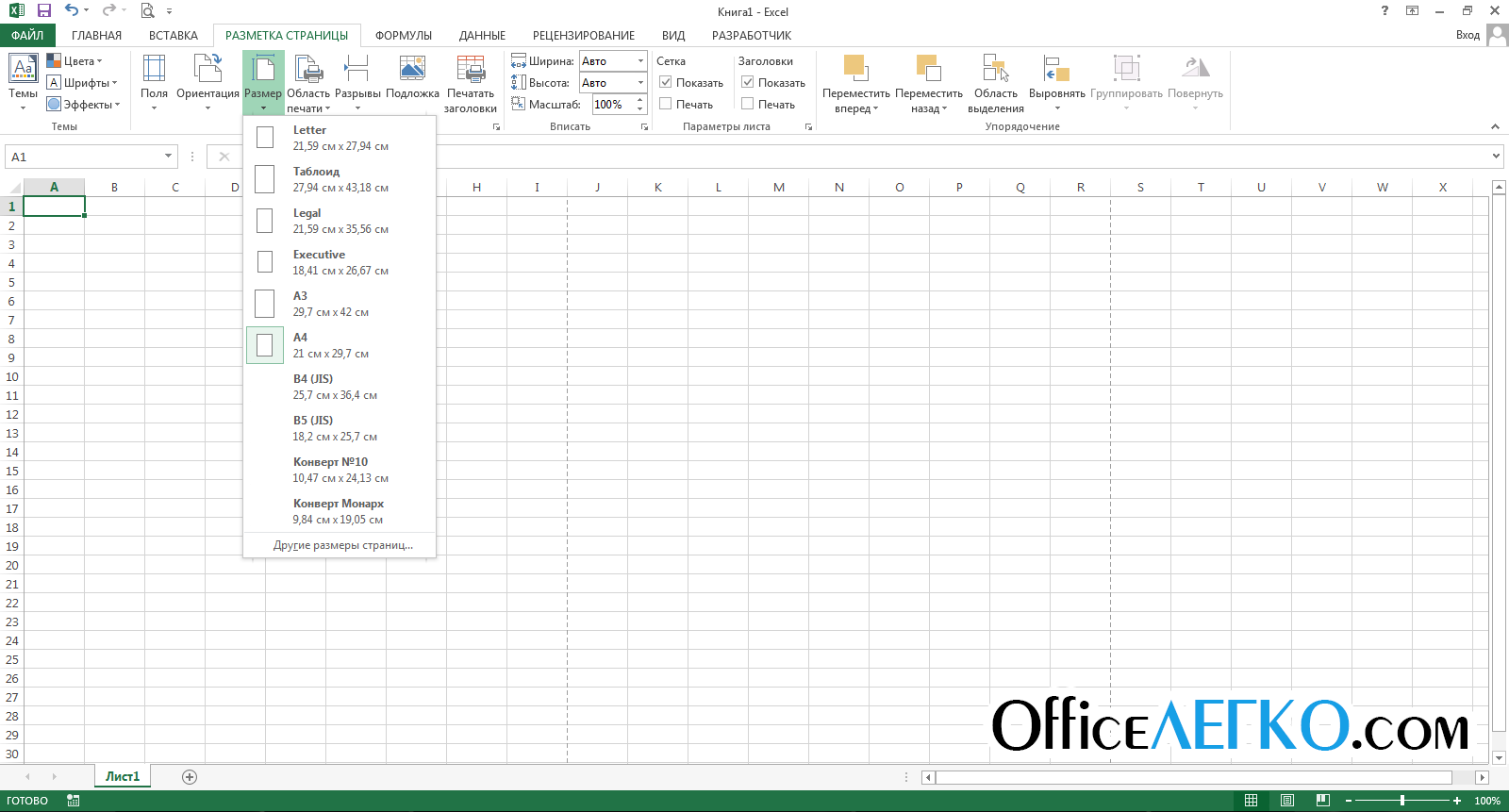
Resizing a sheet in Excel

1. Run File - Print and choose the right size
2. In the window " Page settings» select from list « Paper size»

Setting up fields in Excel

Margins in Excel are empty areas of the page between the edge of the sheet and the border of the cells. There are several ways to customize the margins:

1. Run a tape command Page Layout - Page Setup - Margins . A menu will open to select one of the field options. Alternatively, you can click " Custom fields…' to set dimensions manually

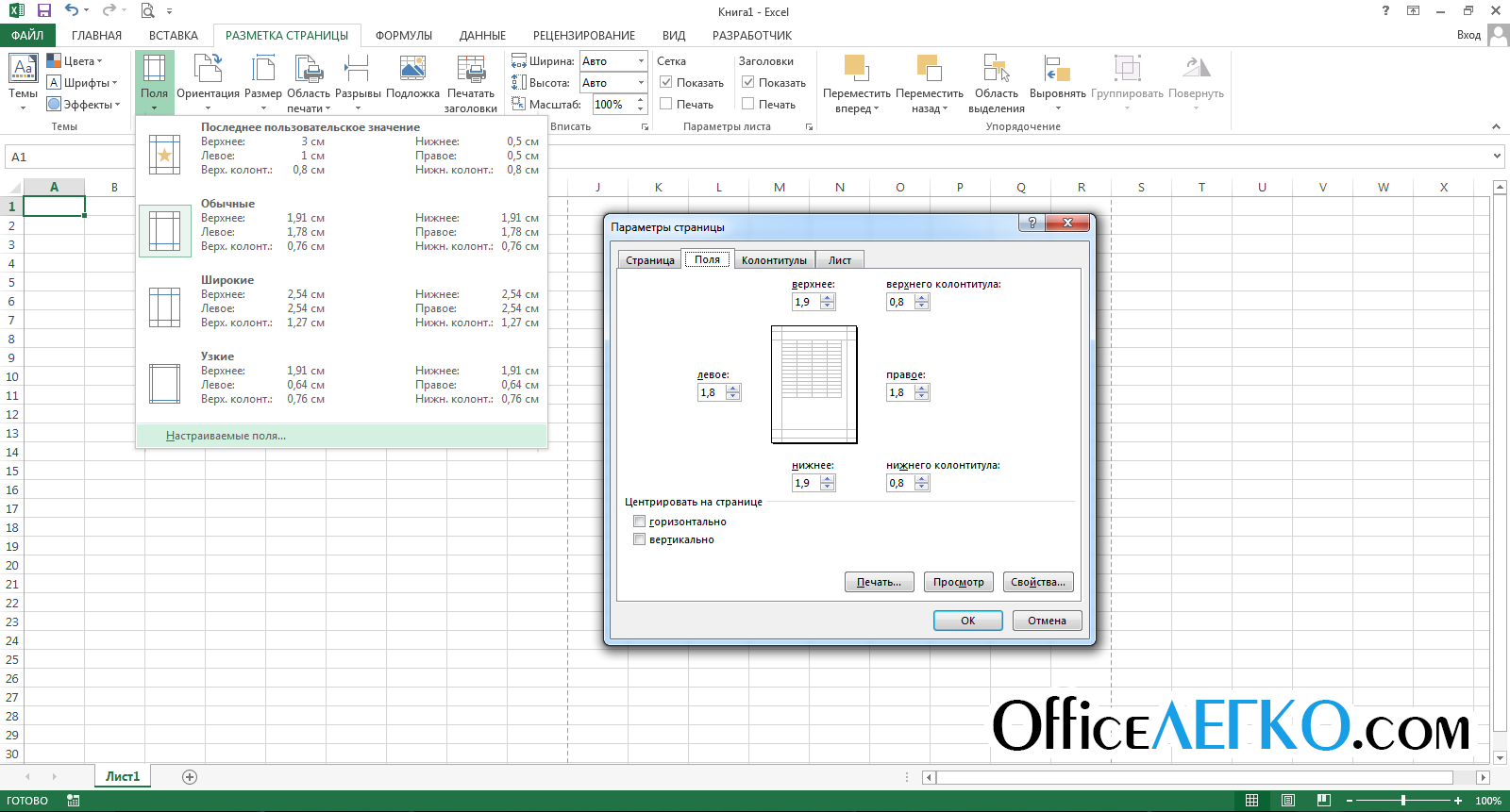
Setting fields in Excel

1. Complete File - Print , in the corresponding section there is a similar menu
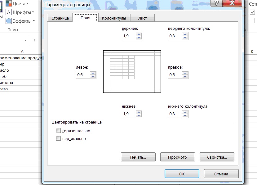
2. Call up the window « Page settings' and go to the tab ' fields» for fine tuning. Here you can manually specify the size of the left, right, top and bottom margins, as well as the headers and footers. Here you can also center the workspace relative to the fields by checking the appropriate checkboxes (the new position will be indicated on the thumbnail in the center of the sheet).

Add headers and footers in Excel

Headers and footers are information areas at the top and bottom of the page in the margins. Headers and footers are repeated on each printed page, supporting information is written in them: page number, author's name, report title, etc. There are three fields for headers and footers (left, center and right) at the top and bottom of the page.

Headers and footers in Microsoft Excel

Yes insert headers and footers - go to, because. header and footer areas are clearly highlighted here. Click inside one of the headers and write informative text. At the same time, the ribbon tab " Working with headers and footers”, which contains additional commands.

Yes, you can insert automatic header and footer, which will indicate the current page number, number of pages per sheet, file name, etc. To insert an automatic element, select it on the ribbon: Working with headers and footers - Constructor - Header and footer elements . These elements can be combined with each other and with free text. To insert - place the cursor in the header and footer field and click on the icon in the "Header and footer elements" group (see figure).

On the Design tab, you can set additional parameters for headers and footers:

• Custom header for the first page- headers and footers of the first page are not repeated on other pages. It is convenient if the first page is the title page.
• Different headers and footers for odd and even pages– suitable for page numbering when printing a booklet
• Scale with the document- the setting is enabled by default, headers and footers are scaled the same way as the entire page. I recommend keeping this option enabled to ensure the integrity of the sheet layout.
• Align with page margins– the left and right headers and footers are aligned to the respective margins. This parameter is also set by default, it makes little sense to change it.

Headers and footers are a handy tool for giving final touch his work. The presence of high-quality, informative headers and footers is a sign of the professionalism of the performer.

Insert a page break in Excel

If you need to insert in some place of the sheet forced break page, position the cursor in the cell on the right below the break and execute the ribbon command Page Layout - Page Setup - Breaks - Insert Page Break. For example, to insert a break after column D and row #10, select cell E11 and run the following command.

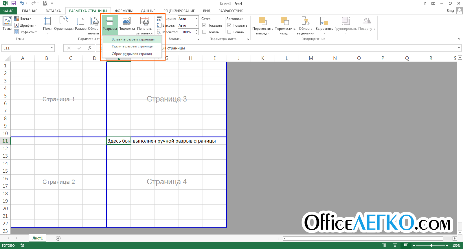
Insert a page break

To remove the gap - there is a reverse command: the command Page Layout - Page Setup - Breaks - Remove Page Break . To remove all manual breaks, there is a command Page Layout - Page Setup - Breaks - Reset Page Breaks .

After inserting a break, page separators will appear on the sheet. In they take the form of blue frames, dragging which, you can change the printed page borders.

Adding a Header in Excel

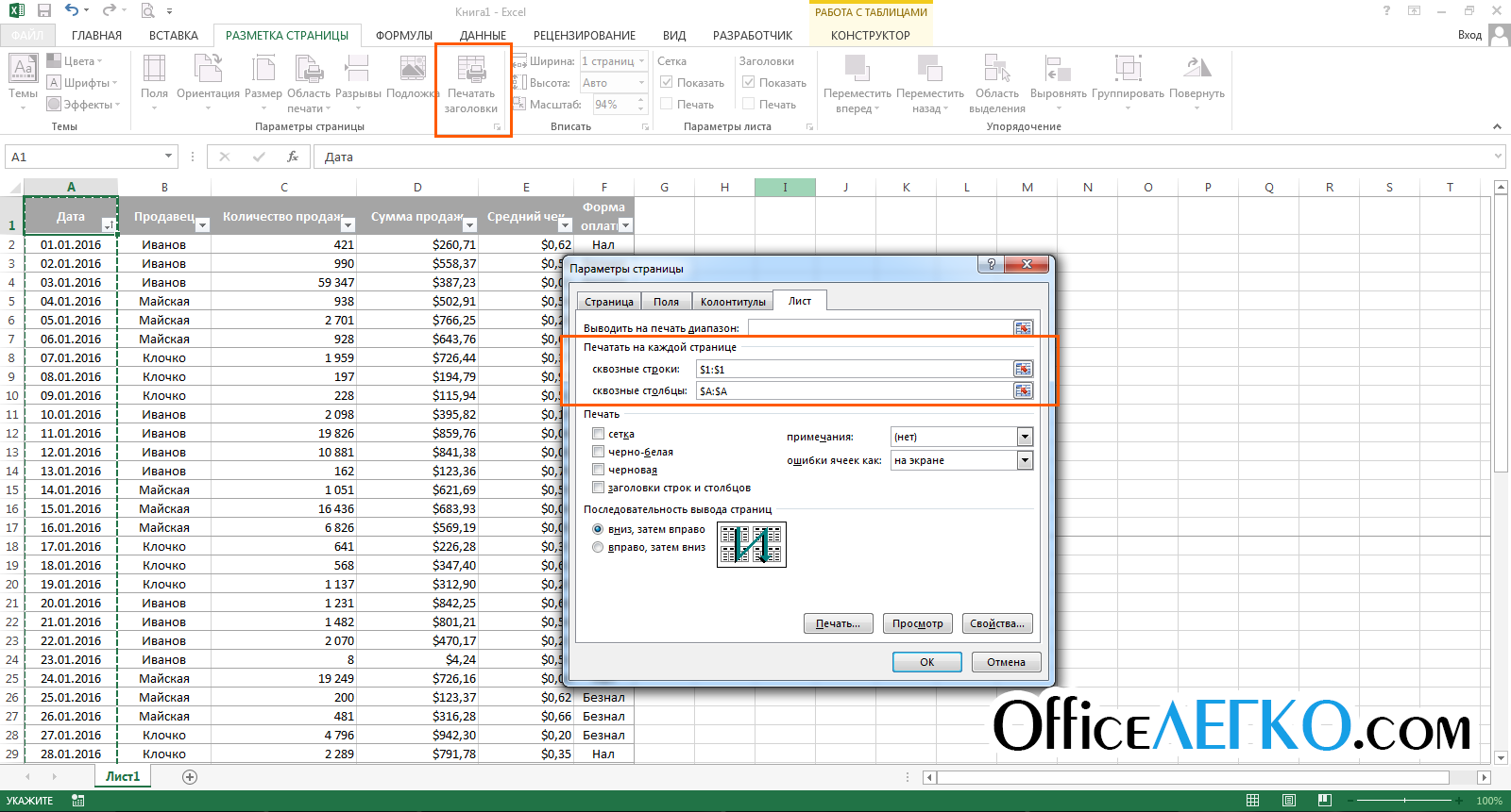
When you print large tables, you want the table header to repeat on every page. If you used , then this function will not affect the header in any way when printing, it will be printed only on the first page.

To have cells repeat on every printed page, run the ribbon command Page Layout - Page Setup - Print Headers . The window " Page settings", tab " Sheet". In this window, in the fields " through lines" And " Through columns» Provide row and column references to repeat on each worksheet. Please note that the selected cells will not be physically present on each page, but will only be repeated when printed.

Adding Headings to Excel

Customize in excel scale printing

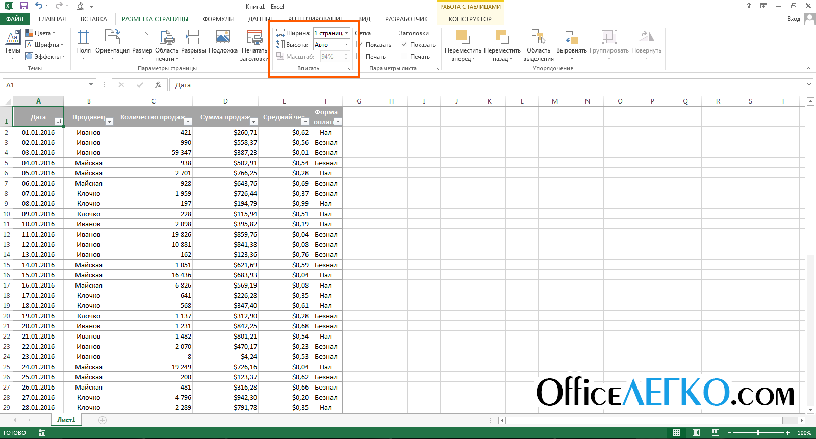
Sometimes the information on the sheet cannot be placed compactly so that it fits on the required number of pages. It is not always convenient to match the column width and row height to get a well-composed sheet. Much more convenient change print scale(not to be confused with display scale). Using this option, you change the scale of your data on the printed page.

To change the print scale, use the ribbon commands Page Layout - Fit . You can set the scale manually using the "Scale" counter, but it is much easier and faster to use the drop-down lists " Width" And " Height". Thanks to them, you can set how many sheets in width and height you will have. For example, to fit data into one page in width, set: Width - 1 page; Height - Auto.

Excel print scale

Hiding before printing

If you do not need to print some data, you can simply hide it. For example, containing technical information, leave only significant data. Most often, reports should not contain details of calculations, but only display their results and conclusions, suggesting certain management decisions.

You can also make objects non-printable. To do this, select it and right-click on the object frame. From the context menu select " Format…". In the dialog box that opens, in the Properties group, uncheck Print an object.

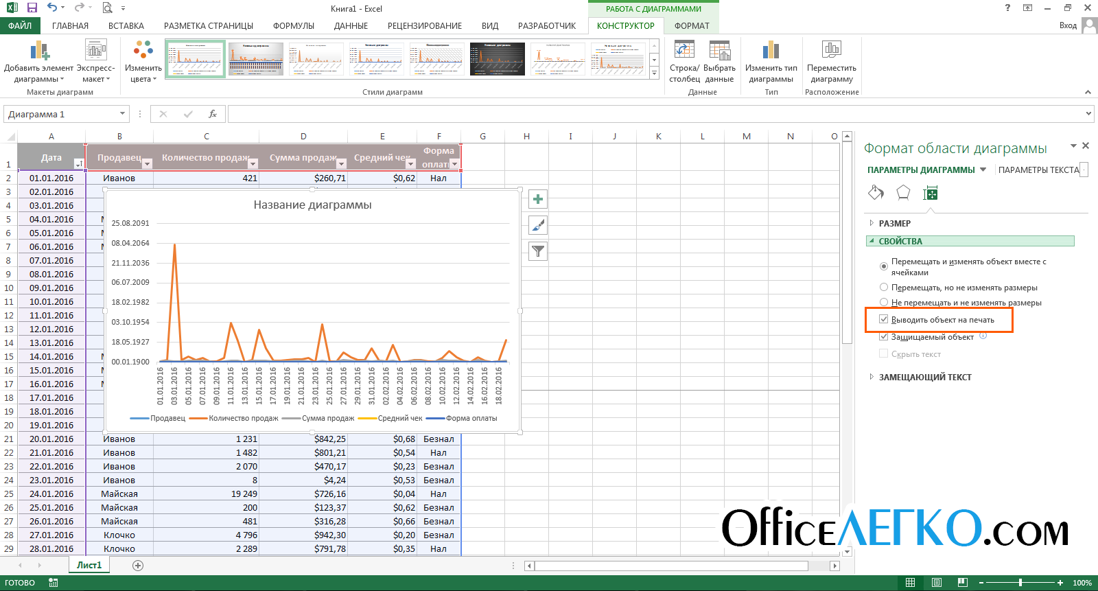
Configuring Printing Excel Objects

Views in Excel

If you use the same document with different display layouts, you will often need to change the same display and formatting options. For example, you update the source data and calculations daily, which you then hide when printing. Instead, you can create multiple views of the same sheet, after which changing the display takes a couple of seconds and a few clicks.

That is, views in Excel are saved formatting and display settings that can be applied at any time, instead of doing it manually. The program saves the following formatting settings in views:

1. worksheet
2. Worksheet settings for printing
3. and cursor position
4. Pinned areas

After you have done all the listed settings, run the command View - Book View Modes - Views - Add . In the Add View window that opens, specify a name for the new view and make your selection from the suggested refiners. Click " OK”, and the view is created!

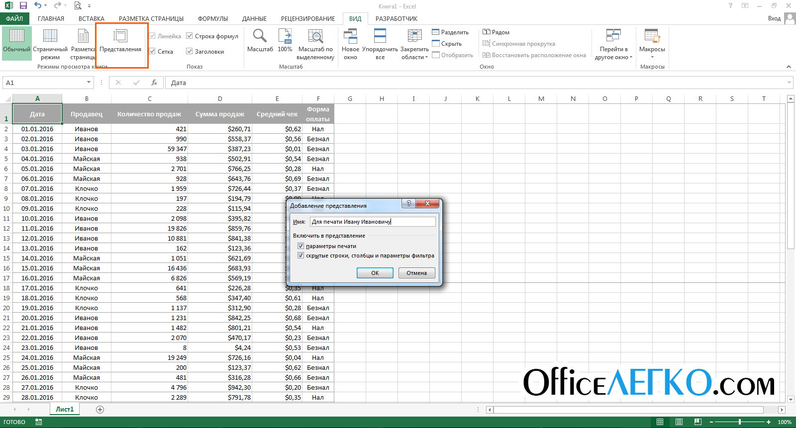
Adding a View to Excel

In the future, to apply the saved view to the workbook, run View - Book Views - Views , select from the list desired representation and press " Apply". Unfortunately, views don't work if the sheet has , which limits the use of the tool.

These are the sheet settings that can and should be done in preparation for printing (and not only). Set up your workbooks the right way so your reports look perfect. Even the highest quality calculations look boring and useless if they are not formatted and prepared for printing. Even if you send out reports by mail, most likely the manager will want to print them. Therefore, I recommend preparing for printing each sheet of the report, regardless of the method of submission for consideration!

Friends, if you still do not understand any details on the materials of the post, ask questions in the comments. And do not forget to subscribe to updates , become professionals with the site ! Always yours, Alexander Tomm

18 comments

Hello, what solution can be found for the following case? Eat big table(more than 3 sheets) and is at the end of the signature officials. When printing, not the entire table is displayed, but its segment of an indefinite length. Maybe less than a page, maybe more than 2. In this case, the signatures must also be. But since the length is not determined in advance, then a situation may turn out when the signatures end up on different pages. If you put a forced break, it may turn out that there is one line in the table, and the signatures are on another page, which is also unsightly. Is it possible to solve automatically, without operator intervention at each print? Thanks in advance

1. Vladimir, you can try to insert signatures in the headers and footers, but it will not work out very well. Or, solve the problem using VBA, but the best way out will still control the eyes of the preprint