Grouping data
When you prepare a catalog of products with prices, it would be nice to take care of the usability of it. A large number of positions on one sheet forces the use of a search, but what if the user only makes a choice and has no idea about the name? In Internet catalogs, the problem is solved by creating product groups. So why not do the same in an Excel workbook?
Grouping is pretty easy. Select multiple lines and click the button Group tab Data(see fig. 1).
Figure 1 - Group button
Then specify the type of grouping − line by line(see Fig. 2).

Figure 2 - Selecting the type of grouping
As a result, we get ... not what we need. Rows of products have been combined into a group indicated below them (see Fig. 3). In directories, the title usually comes first, and then the content.

Figure 3 - Grouping rows "down"
This is by no means a program error. Apparently, the developers considered that the grouping of lines is mainly done by the compilers of financial statements, where the final result is displayed at the end of the block.
To group rows "up" you need to change one setting. On the tab Data click on the small arrow in the lower right corner of the section Structure(see Fig. 4).
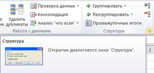
Figure 4 - The button responsible for displaying the structure settings window
In the settings window that opens, uncheck the box. Totals in rows below data(See Fig. 5) and press the button OK.
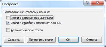
Figure 5 - Structure settings window
All groups that you managed to create will automatically change to the "upper" type. Of course, the set parameter will affect the further behavior of the program. However, you will need to uncheck this box to everyone new sheet and each new Excel workbook, because the developers did not provide for a "global" setting of the grouping type. Similarly, you cannot use Various types groups within the same page.
Once you've sorted your products into categories, you can organize the categories into larger sections. In total, up to nine levels of grouping are provided.
The inconvenience when using this function is the need to press the button OK in a pop-up window, and it will not be possible to collect unrelated ranges in one go.
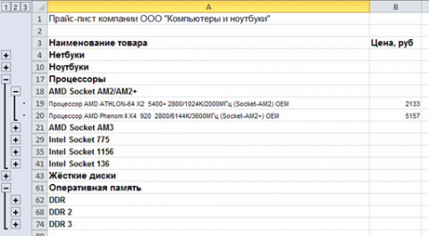
Figure 6 - Multilevel directory structure in Excel
Now you can open and close parts of the catalog by clicking on the pros and cons in the left column (see Figure 6). To expand the entire level, click on one of the numbers at the top.
To output lines for more high level hierarchy, use the button Ungroup tabs Data. You can completely get rid of grouping using the menu item Delete Structure(See Fig. 7). Be careful, it is impossible to undo the action!
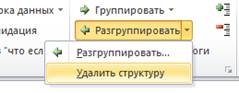
Figure 7 - Removing the grouping of rows
Pinning sheet regions
Quite often when working with Excel spreadsheets there is a need to fix some areas of the sheet. There may be, for example, row / column headings, a company logo or other information.
If you freeze the first row or the first column, then everything is very simple. Open a tab View and drop down menu To fix areas select items accordingly Pin top line or Freeze first column(see fig. 8). However, at the same time, both the row and the column cannot be “frozen” in this way.
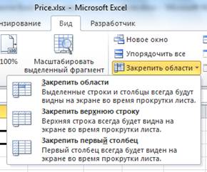
Figure 8 - Freeze a row or column
To remove a pin, select the item in the same menu. Unpin areas(paragraph replaces the line To fix areas if the page has a freeze applied).
But fixing several rows or an area of rows and columns is not so transparent. You highlight three lines, click on an item To fix areas, and... Excel freezes only two. Why is that? An even worse scenario is possible when the regions are fixed in an unpredictable way (for example, you select two lines, and the program puts borders after the fifteenth). But let's not write this off as an oversight by the developers, because the only correct use case for this feature looks different.
You need to click on the cell below the rows you want to freeze, and, accordingly, to the right of the columns to be fixed, and only then select the item To fix areas. Example: in Figure 9, a cell is selected B4. This means that three rows and the first column will be fixed, which will remain in place when the sheet is scrolled both horizontally and vertically.
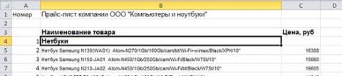
Figure 9 - We fix the area of \u200b\u200brows and columns
You can apply a background fill to anchored areas to indicate to the user that these cells have special behavior.
Sheet rotation (replacing rows with columns and vice versa)
Imagine this situation: you worked for several hours on a set of a table in Excel and suddenly realized that you had designed the structure incorrectly - column headings should have been written in rows or rows in columns (it does not matter). Retype everything manually? Never! Excel provides a function that allows you to "rotate" the sheet by 90 degrees, thus moving the contents of the rows into columns.
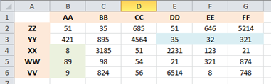
Figure 10 - Initial table
So, we have some table that needs to be “rotated” (see Fig. 10).
- Select cells with data. It is the cells that are selected, not the rows and columns, otherwise nothing will work.
- Copy them to the clipboard with a keyboard shortcut
or in any other way. - Let's move on to empty sheet or free space current sheet. Important note: pasting over the current data is not allowed!
- Paste data with keyboard shortcuts
and select the option from the paste options menu Transpose(see fig. 11). Alternatively, you can use the menu Insert from tab home(see fig. 12).
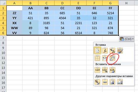
Figure 11 - Insert with transposition
![]()
Figure 12 - Transpose from the main menu
That's it, the rotation of the table is done (see Fig. 13). In this case, the formatting is preserved, and the formulas are changed in accordance with the new position of the cells - no routine work is required.
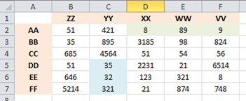
Figure 13 - Result after rotation
Formula display
Sometimes a situation arises when you cannot find the desired formula among a large number of cells, or you simply do not know what and where to look for. In this case, you will need the ability to display not the result of calculations, but the original formulas on the sheet.
Click the button Show formulas tab Formulas(See Figure 14) to change how data is presented on the sheet (See Figure 15).
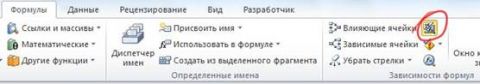
Figure 14 - Button "Show formulas"
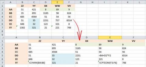
Figure 15 - Now formulas are visible on the sheet, and not the results of the calculation
If you find it difficult to navigate the cell addresses displayed in the formula bar, click Influencing cells from tab Formulas(see fig. 14). Dependencies will be shown with arrows (see Fig. 16). To use this feature, you must first highlight one cell.
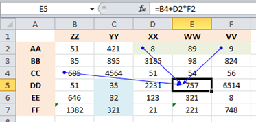
Figure 16 - Cell dependencies are shown by arrows
Hide dependencies at the click of a button Remove arrows.
Wrap lines in cells
Quite often in Excel books there are long labels that do not fit in the cell in width (see Fig. 17). You can, of course, expand the column, but this option is not always acceptable.
Figure 17 - Labels do not fit in cells
Select cells with long labels and click the button Text wrap on Home tab (see Figure 18) to switch to multi-line display (see Figure 19).
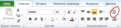
Figure 18 - Button "Wrap Text"

Figure 19 - Multiline text display
Rotate text in a cell
Surely you have come across a situation where the text in the cells needed to be placed not horizontally, but vertically. For example, to label a group of rows or narrow columns. Excel 2010 provides tools to rotate text in cells.
Depending on your preferences, you can go two ways:
- First create an inscription, and then rotate it.
- Adjust the rotation of the label in the cell, and then enter the text.
The options differ slightly, so we will consider only one of them. First, I combined six lines into one using the button Merge and center on Home tab (see Fig. 20) and introduced a generalizing inscription (see Fig. 21).
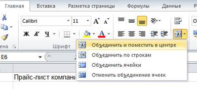
Figure 20 - Merge cells button
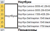
Figure 21 - First create a horizontal signature
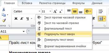
Figure 22 - Text rotation button
You can further reduce the column width (see Figure 23). Ready!
Figure 23 - Vertical cell text
If there is such a desire, you can set the angle of rotation of the text manually. In the same list (see Fig. 22), select the item Cell alignment format and in the window that opens, set an arbitrary angle and alignment (see Fig. 24).
Figure 24 - Set an arbitrary angle of text rotation
Format cells by condition
Possibilities conditional formatting appeared in Excel for a long time, but by the 2010 version they have been significantly improved. You may not even have to understand the intricacies of creating rules, because. the developers have provided a lot of blanks. Let's see how to use conditional formatting in Excel 2010.
The first thing to do is select the cells. Next, on Home tab click Conditional Formatting and select one of the blanks (see Fig. 25). The result will be displayed on the sheet immediately, so you do not have to go through the options for a long time.
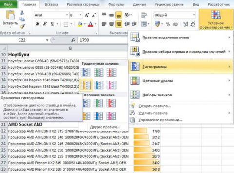
Figure 25 - Selecting a conditional formatting template
Histograms look quite interesting and well reflect the essence of price information - the higher it is, the longer the segment.
Color scales and icon sets can be used to indicate various states, such as transitions from critical to eligible costs (see Figure 26).
Figure 26 - Color scale from red to green with yellow in between
You can combine bar charts, bars, and icons in the same cell range. For example, the bar graphs and icons in Figure 27 show acceptable and excessively poor device performance.
Figure 27 - The histogram and icon set reflect the performance of some conditional devices
To remove conditional formatting from cells, select them and select Conditional Formatting from the menu. Remove rules from selected cells(see fig. 28).
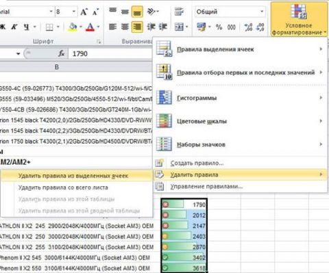
Figure 28 - Delete conditional formatting rules
Excel 2010 uses presets for quick access to the possibilities of conditional formatting, as setting your own rules is far from obvious for most people. However, if the templates provided by the developers do not suit you, you can create your own rules for the design of cells by various conditions. Full description This functionality is beyond the scope of this article.
Using filters
Filters allow you to quickly find the information you need big table and represent it in a compact form. For example, from long list books, you can choose the works of Gogol, and from the price list of a computer store - Intel processors.
Like most other operations, the filter requires cells to be selected. However, you do not need to select the entire table with data, it is enough to mark the rows above the desired data columns. This greatly increases the convenience of using filters.
After the cells are selected, on the tab home press the button Sort and filter and select the item Filter(see fig. 29).
Figure 29 - Creating filters
Now the cells will be converted into drop-down lists where you can set the selection options. For example, we are looking for all mentions of Intel in the column Name of product. To do this, select a text filter Contains(see fig. 30).
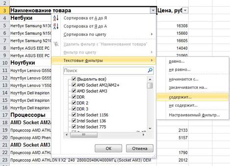
Figure 30 - Creating a text filter
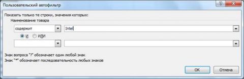
Figure 31 - Create a filter by word
However, it is much faster to achieve the same effect by typing a word in the field Search context menu shown in Figure 30. Why then call an additional window? It is useful if you want to specify several selection conditions or select other filtering options ( does not contain, starts with... ends with...).
Other options are available for numeric data (see Figure 32). For example, you can choose the 10 largest or 7 the smallest values(quantity is customizable).
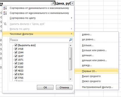
Figure 32 - Numeric filters
Excel filters provide rich enough features, comparable to the selection of a SELECT query in database management systems (DBMS).
Information curve display
Information curves (info curves) - an innovation in Excel 2010. This function allows you to display the dynamics of changes in numerical parameters directly in the cell, without resorting to charting. Changes in numbers will be immediately shown on the micrograph.
Figure 33 - Excel 2010 InfoCurve
To create an infocurve, click one of the buttons in the block Infocurves tab Insert(see Fig. 34), and then set the range of cells to plot.
Figure 34 - Inserting an infocurve
Like charts, information curves have many options to customize. More detailed guide on the use of this functionality is described in the article.
Conclusion
The article discussed some useful Excel features 2010, accelerating work, improving appearance tables or usability. It doesn't matter if you create the file yourself or use someone else's - in Excel 2010 there are functions for all users.
We have repeatedly spoken about spreadsheet editor from Microsoft - Excel program. The entire package of office programs is rightfully the market leader. And this leadership is quite easily explained by the presence of huge functionality. Moreover, with each version it is replenished.
In fact, about a tenth of all functions are not used by an ordinary user, so many do not even know about their existence and do manually what can be done automatically. Or they spend time adjusting to certain limitations and inconveniences. Today we want to tell you about how to fix an area in Excel. In other words, the program has a function thanks to which you can fix the document header for your convenience.
We fix the area (header) in Microsoft Excel
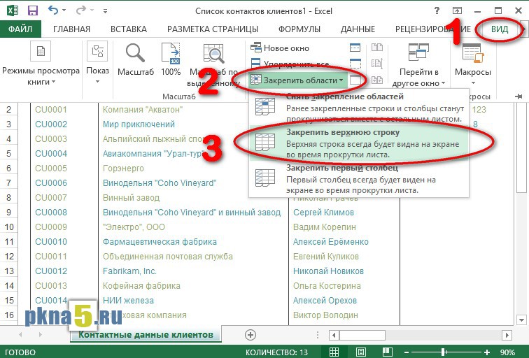
Well, we won't pull any more. Let's go through the process of pinning the area you need as a fixed header that will always stay on top (or side), wherever you scroll the document. So, you must do the following to achieve the desired result:- First of all, go to the "View" tab, then click on the "Freeze Areas" button;
- Now you have to choose the desired pinning option. There are only three of them:
Thus, the choice of a particular item depends solely on your needs.
Freeze both rows and columns at the same time
Be that as it may, these options are only suitable if you want to select one row or one column anywhere in the document. But what if you need to freeze both a row and a column at once so that they are displayed permanently? Let's figure it out: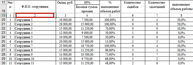
As you can see, there is nothing complicated in both cases. This is literally a matter of minutes. That is why the MS Office office suite (including Excel) is indeed the most popular software for editing all types of text and graphic data: any action can be automated or simplified as much as possible, the main thing is to remember how everything is done.
This instruction is relevant not only for Excel 2013, on which it was demonstrated, but also for older ones - the difference may be in the arrangement of elements, nothing more. Therefore, if you have a different version, do not be too lazy to make a couple of extra mouse movements.
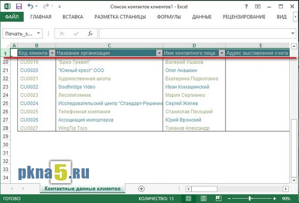
In this material, the answer is on how to freeze a row in excel. We will see how to freeze the first (top) or arbitrary row, and we will also analyze how to freeze an area in excel.
Freezing a row or column in Excel is an extremely useful feature, especially for creating lists and tables with big amount data placed in cells and columns. By pinning a row, you can easily keep track of the headings of certain columns, which means you will save time instead of endlessly scrolling up and down.
Consider an example. In the figure below, we see the first row, which is the column headings.
Agree, it will be inconvenient for us to enter and read data from the table if we do not know or see the headings at the top. Therefore, we fix the upper term in excel in the following way. In the top menu of Excel, we find the "VIEW" item, in the opening submenu, select "LOCK AREAS", and then select the "LOCK TOP ROW" sub-item.
These simple actions to fix the line allow you to scroll through the document and at the same time understand the meaning of the line headers in Excel. I repeat - it is convenient when a large number of lines.
I must say that the same effect can be achieved if you first select the cells of the entire first row, and then apply the first sub-item of the already known submenu "FIX AREAS" - "Freeze areas":
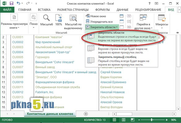
Well, now about how to fix an area in excel. First, select the area of Excel cells that you want to permanently see (pin). It can be several lines and an arbitrary number of cells. As you probably already guess, the path to this pinning function remains the same: menu item "VIEW" → further "LOCK AREAS" → further sub-item "LOCK AREAS". This is illustrated in the top figure.
If for some reason you were not able to properly freeze rows or areas in excel, go to the "VIEW" menu → "FREEZE AREAS" → select "Unfreeze areas". Now you can again try to slowly fix the desired lines and areas of the document.
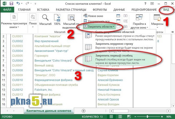
Finally, I will say that the first column can also be fixed. We also act → menu "VIEW" → "LOCK AREAS" → select the item "Freeze first column".
Good luck with working with documents in Excel, do not make mistakes and save your time by using the additional features and tools of this editor.